1. To find the y-intercept:
Hit  , #5 TRACE, #1 Graph Trace. The spider will start on the y-axis,
showing the y-intercept. |
|
2. To find the x-intercept:
The x-intercept of a graph is also known as the "root" or the "zero" of the function.
Press MENU - #5 - #1 to TRACE the graph.
Use the NavPad to move the trace point to the x-axis. As you approach the x-axis, the spider will "jump" to the zero location. When the  appears, you have found a zero of the function. appears, you have found a zero of the function.
Read more about Zeros. |
|
3. To find where the graphs intersect:
A second graph is plotted  . .
Press MENU - #6 Points & Lines - #3 Intersection Points
When the pointing hand appears, click on each graph
and all intersections points will be found.
Read more about Intersection Points |
|
4. To find a specific value while tracing:
To "jump" to a certain x-coordinate on the screen,
press MENU - #5 Trace - #1 Graph Trace - Enter.
Now, simply type the x-coordinate that you desire.
The ordered pair will appear and the spider will be located at the closest plotable point.
If you choose a value out of the current viewing window, the graph will adjust to include your new point.
For this graph, the x-coordinate 22 was selected. Notice the dotted line indicating the location on the x-axis as well as the ordered pair (22,-8).
|
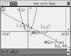 Up and down arrows will move between functions.
 |
5. Controlling what the graph looks like (attributes):
Be sure the command line is referring to the graph you wish to alter.
Press  to move along the options on the command (entry) line. to move along the options on the command (entry) line.
The  is the Hide/Show button. is the Hide/Show button.
The  is the Attribute button. The attributes appear below. is the Attribute button. The attributes appear below. |
|
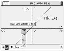 Line Weight: Thin,
Medium,
Thick
 |
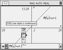 Line Style: Solid, Dashed, Dotted
 |
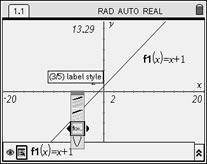 Label Style: y =, f( ), f( )=, y = f( ), f
 |
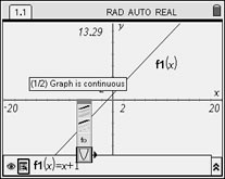 Continuous or Discrete
 |
|
|


![]()